
| 일 | 월 | 화 | 수 | 목 | 금 | 토 |
|---|---|---|---|---|---|---|
| 1 | 2 | 3 | 4 | 5 | 6 | |
| 7 | 8 | 9 | 10 | 11 | 12 | 13 |
| 14 | 15 | 16 | 17 | 18 | 19 | 20 |
| 21 | 22 | 23 | 24 | 25 | 26 | 27 |
| 28 | 29 | 30 | 31 |
- 이력서 첨삭
- 주요 파라미터
- 경력기술서 첨삭
- 데이터 사이언티스트
- 판다스
- 머신러닝
- 주식데이터
- 데이터 분석
- 코딩테스트
- 과제전형
- 데이터분석
- 사이킷런
- 퀀트
- 데이터 사이언스
- sklearn
- 하이퍼 파라미터 튜닝
- 데이터사이언스
- 대학원
- 하이퍼 파라미터
- 경력 기술서
- AutoML
- 파이썬
- 커리어전환
- 주가데이터
- 데이터사이언티스트
- 랜덤포레스트
- pandas
- 공공데이터
- 자기소개서
- 퀀트 투자 책
- Today
- Total
GIL's LAB
실험 7. 골든크로스와 데드크로스의 효과 분석 본문
개요
이번 실험에서는 골든크로스가 발생하면 주가가 상승하고, 데드크로스가 발생하면 주가가 하락하는지를 확인해보고자 한다.
먼저, 골든크로스와 데드크로스가 무엇인지 설명하자.
골든크로스와 데드크로스는 모두 이동평균선이 교차하는 지점이다.
골든크로스는 단기 이동 평균선이 올라가고 장기 이동 평균선이 내려가면서 두 이평선이 교차하는 것으로, 최근 주가가 과거보다 상승하고 있다는 신호로 알려져 있다. 반대로, 데드크로스는 장기 이동 평균선이 올라가고 단기 이동 평균선이 내려가면서 두 이평선이 교차하는 것으로, 최근 주가가 과거보다 하락하고 있다는 신호로 알려져있다.
이동평균선 혹은 이평선은 특정 기간동안의 평균 주가를 의미하며, 5일, 10일 이평선을 보통 단기 이동 평균선, 60일, 120일 이평선을 중장기 이동 평균선이라 한다.
시계열 개념이 친숙하다면, moving average와 같은 의미라고 받아들이면 된다.
아래 이미지에서 보는 것처럼, 골든크로스와 데드크로스 모두 빨간색 단기이평선과 초록색 장기이평선이 만나는 점인데, 골든크로스는 단기이평선이 올라가면서 만나는 점이고, 데드크로스는 단기이평선이 내려가면서 만나는 점이다.

실험 내용
이번 실험에서는 골든크로스 지점에서 매수를 하고, 데드크로스 지점에서 매도를 하는 것이 정말로 효과적인 투자 전략인지를 검증하고자 한다.
구체적인 내용은 다음과 같다.
- 골든크로스 지점에서 매수하고 바로 이어지는 데드크로스 지점에서 매도했을 때의 기대 수익 계산
- 골든크로스 지점에서 매수하고 1, 3, 6, 12개월 후 매도했을 때의 기대 수익 계산
- 데드크로스 지점에서 매수하고 1, 3, 6, 12개월 후 매도했을 때의 기대 수익 계산
데이터 준비 및 전처리
그러면 곧바로 파이썬 코드로 가보자.
먼저 필요한 모듈을 불러온다.
# 모듈 불러오기
import pandas as pd
import os
import warnings
import numpy as np
import itertools

warnings.filterwarnings("ignore")
그리고 주가 데이터가 있는 경로를 설정하고, 데이터를 담을 사전을 정의한다.
path = "../../QUANT_DATA/201609~202108/주가/일"
data_dict = dict()
데이터를 모두 불러온 뒤에 전처리를 하면 불필요한 단계가 포함될 수 있어서, 데이터를 불러오면서 전처리를 하고, 전처리한 데이터를 data_dict에 저장할 것이다.
전처리 및 검증을 위해 필요한 함수들을 하나하나 정의하자.
먼저, 주가 데이터(data)에서 날짜(date)를 입력했을 때, 해당 날짜의 주가 혹은 해당 날짜와 가장 가까운 날짜의 주가를 가져오는 함수를 정의한다.
def get_nearest_close_price(data, date):
    # data에서 날짜가 date일 때의 종가 가져오기
    # 단, date일 때 장이 열리지 않았다면, 가장 최근에 열린 장의 데이터를 사용
    # 예: 2021년 10월 2일 가격이 없으면 10월 1일 가격을 가져옴
    while True:
        if date in data.index:
            return data.loc[date, '종가']
            break
        else:
            date = date - pd.to_timedelta(1, unit = "D")
그리고 골든크로스인지 데드크로스인지를 나타내는 함수를 정의한다.
두 함수 모두 단기이평선(short_term_MA)와 장기이평선(long_term_MA)를 입력으로 받는다.
그리고 i번째 시점에서 단기이평선이 장기이평선 위에 있는데, 직전 시점에서 장기이평선이 단기이평선 위에 있다면 골든 크로스라고 판단하고, 그 반대의 경우에는 데드크로스로 판단한다.
두 함수의 리턴값은 해당 시점에서 골든크로스(데드크로스)면 True를, 그렇지 않으면 False를 반환하는 부울 배열이다.
def goldencross(short_term_MA, long_term_MA):
    result = [False]
    for i in range(1, len(short_term_MA)):
        if (short_term_MA.iloc[i] >= long_term_MA.iloc[i]) and (short_term_MA.iloc[i-1] < long_term_MA.iloc[i-1]):
            result.append(True)
        else:
            result.append(False)

    return result
def deadcross(short_term_MA, long_term_MA):
result = [False]
for i in range(1, len(short_term_MA)):
if (short_term_MA.iloc[i] <= long_term_MA.iloc[i]) and (short_term_MA.iloc[i-1] > long_term_MA.iloc[i-1]):
result.append(True)
else:
result.append(False)
return result이제 주가 데이터를 전처리하는 함수를 만들자.
코드가 길지만, 내용은 단순하다.
먼저, 날짜라는 컬럼에 YYYYMMDD 형식으로 날짜가 정의되어 있는데, 숫자로 인식되어 있다.
이를 문자로 치환하여 YYYY, MM, DD를 가져오고, 날짜를 datetime으로 정의한 뒤, 날짜를 기준으로 오름차순 정렬하고, 날짜를 인덱스로 설정한다.
그리고 Series의 rolling 메서드를 사용하여 5일, 20일, 60일, 120일 이동 평균을 구한다.
이동평균을 구하는 과정에서 앞 부분에 결측이 생기므로, 결측이 있는 부분을 제거한다.
결측을 제거하고 데이터가 남아있다면, 앞서 정의했던 goldencross, deadcross 함수를 이용하여 골든크로스와 데드크로스 여부를 나타내는 컬럼을 만든다.
사실 골든크로스와 데드크로스의 정의에서 장기와 단기 이평선이 정확히 어떤 이평선인지를 정의하고 있지 않아, 4가지 경우의 수를 모두 고려한다.
그리고 크로스가 포함된 컬럼이 모두 False라면 합이 0일테므로, 이 것을 활용해서 크로스가 없는 데이터라면 None을 리턴한다.
def data_preprocessing(data):
    YYYY = data["날짜"].astype(str).str[:4]
    MM = data["날짜"].astype(str).str[4:6]
    DD = data["날짜"].astype(str).str[6:8]
    data["날짜"] = pd.to_datetime(YYYY + "/" + MM + "/" + DD)
    data.sort_values("날짜", inplace = True) # 날짜를 오름차순으로 정렬
    data.set_index("날짜", inplace = True) # 날짜를 인덱스로 설정

    data['5일이동평균'] = data['종가'].rolling(5).mean()
    data['20일이동평균'] = data['종가'].rolling(20).mean()
    data['60일이동평균'] = data['종가'].rolling(60).mean()
    data['120일이동평균'] = data['종가'].rolling(120).mean()
    data.dropna(inplace = True)

    if len(data) > 0:
        data['5-60_골든크로스'] = goldencross(data['5일이동평균'], data['60일이동평균'])
        data['5-120_골든크로스'] = goldencross(data['5일이동평균'], data['120일이동평균'])
        data['20-60_골든크로스'] = goldencross(data['20일이동평균'], data['60일이동평균'])
        data['20-120_골든크로스'] = goldencross(data['20일이동평균'], data['120일이동평균'])

        data['5-60_데드크로스'] = deadcross(data['5일이동평균'], data['60일이동평균'])
        data['5-120_데드크로스'] = deadcross(data['5일이동평균'], data['120일이동평균'])
        data['20-60_데드크로스'] = deadcross(data['20일이동평균'], data['60일이동평균'])
        data['20-120_데드크로스'] = deadcross(data['20일이동평균'], data['120일이동평균'])

        cross_cols = [col for col in data.columns if '크로스' in col]
        if data[cross_cols].sum().sum() > 0: # 크로스가 하나라도 있어야 함
            return data[cross_cols + ['종가']]
        else:
            return None
    else:
        return None
이제 코스피와 코스닥 데이터를 가져오면서 전처리를 한 뒤, data_dict에 추가한다.
# 데이터 불러오기 및 정제
for market in ["KOSPI", "KOSDAQ"]:
    for file_name in os.listdir(path + "/{}".format(market)):
        df = pd.read_csv(path + "/{}/".format(market) + file_name, encoding = "cp949")
        preprocessed_data = data_preprocessing(df)
        if type(preprocessed_data) != type(None):
            data_dict[file_name.split('.')[0]] = preprocessed_data
골든크로스 지점에서 매수, 데드크로스 지점에서 매도 시 기대 수익 계산
먼저 수익률 목록을 담을 사전을 정의한다.
# 수익률 목록 사전 초기화
profit_list_dict = dict()
그리고 코드 작성의 편의를 위해, 골든크로스 관련 컬럼과 데드크로스 관련 컬럼을 정의한다.
# 컬럼 설정
golden_cross_col_list = ['5-60_골든크로스', '5-120_골든크로스', '20-60_골든크로스', '20-120_골든크로스']
dead_cross_col_list = ['5-60_데드크로스', '5-120_데드크로스', '20-60_데드크로스', '20-120_데드크로스']
이제 모든 (golden_cross_col, dead_cross_col)을 기준으로 매매했을 때의 수익을 계산한다.
itertools.product를 이용하여 먼저 모든 조합을 순회하면서, profit_list를 빈 리스트로 초기화한다.
그 다음으로 해당 컬럼들에 True인 값이 하나라도 있으면, 골든크로스 지점과 데드크로스 지점을 탐색하여 각각 buying_time과 selling_time에 저장한다.
이제 buying_time에 있는 값을 bt로 순회하면서, 이 시점에서의 종가를 buying_price에 정의하고, bt보다 큰 selling_time에 있는 값 가운데 가장 작은 값을 매도 시점으로 정한다.
만약, bt 이후에 데드크로스가 없으면, 데이터가 끝나는 시점에 매도한다.
이 결과를 profit_list에 추가한 뒤, 골든크로스컬럼과 데드크로스 컬럼을 key로 하는 profit_list_dict에 profit_list를 저장한다.
for golden_cross_col, dead_cross_col in itertools.product(golden_cross_col_list, dead_cross_col_list):
    # 수익률 목록 초기화
    profit_list = []
    for key in data_dict.keys():
        data = data_dict[key]
        if data[[golden_cross_col, dead_cross_col]].sum().sum() > 0:
            # 데이터를 순회하면서, 데드크로스와 골든크로스가 존재하는 데이터에 대해서만 아래 작업을 수행

            # 골든크로스 발생 시점을 모두 buying_time에 정의
            # 데드크로스 발생 시점을 모두 selling_time에 정의
            buying_time = data.loc[data[golden_cross_col]].index
            selling_time = data.loc[data[dead_cross_col]].index

            # 모든 골든크로스 발생 시점을 순회하면서
            for bt in buying_time:
                buying_price = data.loc[bt, '종가']
                if sum(selling_time > bt) > 0: # bt보다 이후에 발생한 데드크로스에서 판매
                    st = selling_time[selling_time > bt].min()
                    selling_price = data.loc[st, '종가']
                else: # 만약 이후에 발생한 데드크로스가 없으면, 끝까지 존버하다 판매
                    selling_price = data['종가'].iloc[0]
                profit = ((selling_price - buying_price) / buying_price) * 100
                profit_list.append(profit)

    profit_list_dict[golden_cross_col, dead_cross_col] = profit_list
이제 코드의 결과를 확인하자.
profit_list_dict에 있는 모든 요소에 describe 메서드를 이용하여 통계량을 낸 뒤, 이를 result라는 사전에 추가하고, DataFrame으로 변환하여 출력한다.
result = dict()
for key in profit_list_dict.keys():
    result[key] = pd.Series(profit_list_dict[key]).describe()

pd.DataFrame(result).T
파이썬에서 출력하니 보기가 힘들어서, 엑셀로 정리하였다.
모두 단위가 %임을 생각해서 해석해보도록 하자.
먼저, 최소값은 -95%인 경우가 있는데, 아마도 데드크로스가 발생하지 않고 버티기만 하다가 거의 상장폐지에 가까웠던 종목이 있던게 아닌가라고 추측할 수 있다.
그런데 어떤 골든크로스를 사용하던, 어떤 데드크로스를 사용하던, 50% 이상은 손실을 보게된다.
그러나 평균 이익은 양수로, 손실을 보는 사람은 많지만, 소수의 사람이 이익을 더 많이 보는 전략이라고 볼 수 있다.
전반적으로 따라할만한 전략은 아닌 듯 하다.

골든크로스 지점에서 매수하고 1, 3, 6, 12개월 후 매도했을 때의 기대 수익 계산
수익률 목록을 초기화하고, 골든크로스 관련 컬럼을 정의한다.
# 수익률 목록 사전 초기화
profit_list_dict = dict()
# 컬럼 설정
golden_cross_col_list = ['5-60_골든크로스', '5-120_골든크로스', '20-60_골든크로스', '20-120_골든크로스']이제 각 컬럼을 순회하면서, 골든크로스 지점에서의 가격과 (bt), 1개월, 3개월, 6개월, 1년후의 가격을 비교하여, 수익률을 계산한다.
코드가 굉장히 길지만, 결국 핵심은 골든크로스가 발생한 지점을 buying_time에 정의하고, buying_time에 있는 요소에서 특정 기간 이후에서 시점이 데이터에 포함되어 있는지에 따라 이익을 계산하는 것이다.
그리고 계산한 결과를 기간 차이에 따라, 대응되는 리스트에 추가한다.
for golden_cross_col in golden_cross_col_list:
    # 수익률 목록 초기화
    one_month_profit_list = []
    three_month_profit_list = []
    six_month_profit_list = []
    one_year_profit_list = []

    for key in data_dict.keys():
        data = data_dict[key]
        if data[golden_cross_col].sum() > 0:
            # 골든크로스 발생 시점을 모두 buying_time에 정의
            buying_time = data.loc[data[golden_cross_col]].index

            # 모든 골든크로스 발생 시점을 순회하면서
            for bt in buying_time:
                # 1개월 후 시점, 3개월 후 시점, 6개월 후 시점, 1년 후 시점
                buying_price = data.loc[bt, '종가']
                one_month_st = bt + pd.to_timedelta(30, "D")
                three_month_st = bt + pd.to_timedelta(90, "D")
                six_month_st = bt + pd.to_timedelta(180, "D")
                one_year_st = bt + pd.to_timedelta(365, "D")

                # 현 시점 + 1년 후의 데이터도 존재하면 1개월, 3개월, 6개월, 1년 후 수익 계산
                if one_year_st < data.index.max():
                    one_month_selling_price = get_nearest_close_price(data, one_month_st)
                    three_month_selling_price = get_nearest_close_price(data, three_month_st)
                    six_month_selling_price = get_nearest_close_price(data, six_month_st)
                    one_year_selling_price = get_nearest_close_price(data, one_month_st)

                    one_month_selling_profit = (one_month_selling_price - buying_price) / buying_price * 100
                    three_month_selling_profit = (three_month_selling_price - buying_price) / buying_price * 100
                    six_month_selling_profit = (six_month_selling_price - buying_price) / buying_price * 100
                    one_year_selling_profit = (one_year_selling_price - buying_price) / buying_price * 100

                    one_month_profit_list.append(one_month_selling_profit)
                    three_month_profit_list.append(three_month_selling_profit)
                    six_month_profit_list.append(six_month_selling_profit)
                    one_year_profit_list.append(one_year_selling_profit)

                # 현 시점 + 6개월 후의 데이터도 존재하면 1개월, 3개월, 6개월 후 수익 계산
                elif six_month_st < data.index.max():
                    one_month_selling_price = get_nearest_close_price(data, one_month_st)
                    three_month_selling_price = get_nearest_close_price(data, three_month_st)
                    six_month_selling_price = get_nearest_close_price(data, six_month_st)

                    one_month_selling_profit = (one_month_selling_price - buying_price) / buying_price * 100
                    three_month_selling_profit = (three_month_selling_price - buying_price) / buying_price * 100
                    six_month_selling_profit = (six_month_selling_price - buying_price) / buying_price * 100

                    one_month_profit_list.append(one_month_selling_profit)
                    three_month_profit_list.append(three_month_selling_profit)
                    six_month_profit_list.append(six_month_selling_profit)

                # 현 시점 + 3개월 후의 데이터도 존재하면 1개월, 3개월 후 수익 계산
                elif three_month_st < data.index.max():
                    one_month_selling_price = get_nearest_close_price(data, one_month_st)
                    three_month_selling_price = get_nearest_close_price(data, three_month_st)

                    one_month_selling_profit = (one_month_selling_price - buying_price) / buying_price * 100
                    three_month_selling_profit = (three_month_selling_price - buying_price) / buying_price * 100

                    one_month_profit_list.append(one_month_selling_profit)
                    three_month_profit_list.append(three_month_selling_profit)

                # 현 시점 + 1개월 후의 데이터도 존재하면 1개월 후 수익 계산
                elif one_month_st < data.index.max():
                    one_month_selling_price = get_nearest_close_price(data, one_month_st)
                    one_month_selling_profit = (one_month_selling_price - buying_price) / buying_price * 100
                    one_month_profit_list.append(one_month_selling_profit)

    profit_list_dict[golden_cross_col, "1M"] = one_month_profit_list
    profit_list_dict[golden_cross_col, "3M"] = three_month_profit_list
    profit_list_dict[golden_cross_col, "6M"] = six_month_profit_list
    profit_list_dict[golden_cross_col, "1Y"] = one_year_profit_list
실험 결과는 이전 방법과 동일하게 정리한다.
result = dict()
for key in profit_list_dict.keys():
    result[key] = pd.Series(profit_list_dict[key]).describe()

pd.DataFrame(result).T
의외의 결과가 몇 개 보이니 해석해보도록 하자.
먼저, 골든크로스 지점에 종목을 구매할 것이면 1년이 아니라, 6개월을 보유하는 것이 가장 큰 이익이 됨을 확인했다.
그리고 중위수가 0에 가까웠는데, 딱 절반은 손실을 보고 절반은 이익을 보는 구조라는 것을 알 수 있다.
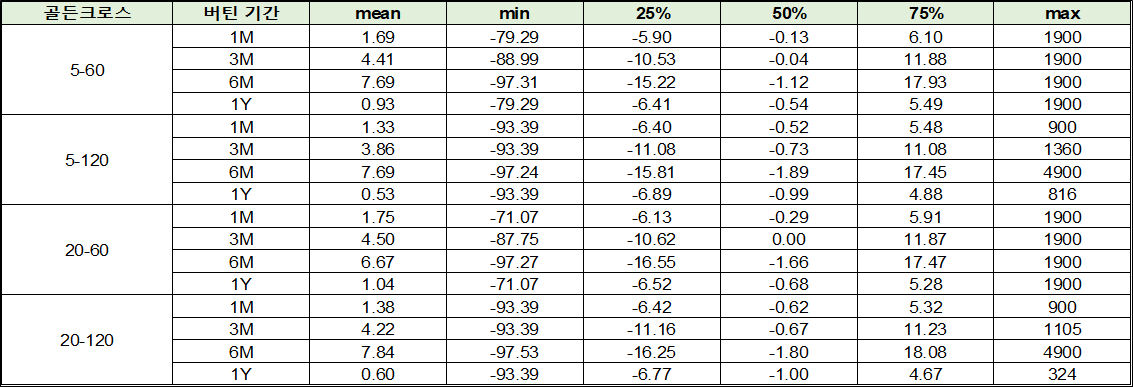
그렇다하더라도 골든크로스 지점에서 구매하는 것은 추천할만한 전략은 아닌 것으로 보인다.
데드크로스 지점에서 매수하고 1, 3, 6, 12개월 후 매도했을 때의 기대 수익 계산
수익률 목록을 초기화하고, 데드크로스 관련 컬럼을 정의한다.
컬럼이 데드크로스와 관련된 것만 빼면, 위의 실험 과정과 완전히 동일하다.
# 수익률 목록 사전 초기화
profit_list_dict = dict()
# 컬럼 설정
dead_cross_col_list = ['5-60_데드크로스', '5-120_데드크로스', '20-60_데드크로스', '20-120_데드크로스']for dead_cross_col in dead_cross_col_list:
# 수익률 목록 초기화
one_month_profit_list = []
three_month_profit_list = []
six_month_profit_list = []
one_year_profit_list = []
for key in data_dict.keys():
data = data_dict[key]
if data[dead_cross_col].sum() > 0:
# 골든크로스 발생 시점을 모두 buying_time에 정의
buying_time = data.loc[data[dead_cross_col]].index
# 모든 골든크로스 발생 시점을 순회하면서
for bt in buying_time:
# 1개월 후 시점, 3개월 후 시점, 6개월 후 시점, 1년 후 시점
buying_price = data.loc[bt, '종가']
one_month_st = bt + pd.to_timedelta(30, "D")
three_month_st = bt + pd.to_timedelta(90, "D")
six_month_st = bt + pd.to_timedelta(180, "D")
one_year_st = bt + pd.to_timedelta(365, "D")
# 현 시점 + 1년 후의 데이터도 존재하면 1개월, 3개월, 6개월, 1년 후 수익 계산
if one_year_st < data.index.max():
one_month_selling_price = get_nearest_close_price(data, one_month_st)
three_month_selling_price = get_nearest_close_price(data, three_month_st)
six_month_selling_price = get_nearest_close_price(data, six_month_st)
one_year_selling_price = get_nearest_close_price(data, one_month_st)
one_month_selling_profit = (one_month_selling_price - buying_price) / buying_price * 100
three_month_selling_profit = (three_month_selling_price - buying_price) / buying_price * 100
six_month_selling_profit = (six_month_selling_price - buying_price) / buying_price * 100
one_year_selling_profit = (one_year_selling_price - buying_price) / buying_price * 100
one_month_profit_list.append(one_month_selling_profit)
three_month_profit_list.append(three_month_selling_profit)
six_month_profit_list.append(six_month_selling_profit)
one_year_profit_list.append(one_year_selling_profit)
# 현 시점 + 6개월 후의 데이터도 존재하면 1개월, 3개월, 6개월 후 수익 계산
elif six_month_st < data.index.max():
one_month_selling_price = get_nearest_close_price(data, one_month_st)
three_month_selling_price = get_nearest_close_price(data, three_month_st)
six_month_selling_price = get_nearest_close_price(data, six_month_st)
one_month_selling_profit = (one_month_selling_price - buying_price) / buying_price * 100
three_month_selling_profit = (three_month_selling_price - buying_price) / buying_price * 100
six_month_selling_profit = (six_month_selling_price - buying_price) / buying_price * 100
one_month_profit_list.append(one_month_selling_profit)
three_month_profit_list.append(three_month_selling_profit)
six_month_profit_list.append(six_month_selling_profit)
# 현 시점 + 3개월 후의 데이터도 존재하면 1개월, 3개월 후 수익 계산
elif three_month_st < data.index.max():
one_month_selling_price = get_nearest_close_price(data, one_month_st)
three_month_selling_price = get_nearest_close_price(data, three_month_st)
one_month_selling_profit = (one_month_selling_price - buying_price) / buying_price * 100
three_month_selling_profit = (three_month_selling_price - buying_price) / buying_price * 100
one_month_profit_list.append(one_month_selling_profit)
three_month_profit_list.append(three_month_selling_profit)
# 현 시점 + 1개월 후의 데이터도 존재하면 1개월 후 수익 계산
elif one_month_st < data.index.max():
one_month_selling_price = get_nearest_close_price(data, one_month_st)
one_month_selling_profit = (one_month_selling_price - buying_price) / buying_price * 100
one_month_profit_list.append(one_month_selling_profit)
profit_list_dict[dead_cross_col, "1M"] = one_month_profit_list
profit_list_dict[dead_cross_col, "3M"] = three_month_profit_list
profit_list_dict[dead_cross_col, "6M"] = six_month_profit_list
profit_list_dict[dead_cross_col, "1Y"] = one_year_profit_list마찬가지로 실험 결과를 확인하자.
result = dict()
for key in profit_list_dict.keys():
    result[key] = pd.Series(profit_list_dict[key]).describe()

pd.DataFrame(result).T
굉장히 당황스러운 결과인데, 사실 데드크로스에서 매수하는 전략은 거의 누구도 하지 않는다.
그런데 데드크로스에서 매수하는거와 골든크로스에서 매수하는것에 큰 차이가 없었고, 심지어는 골든크로스에서 구매해서 데드크로스에서 파는 것보다 데드크로스에서 사서 그냥 묵히는 것이 더 큰 이익이 나는 것을 확인했다.

이번 실험의 결론은 막연히 데드크로스, 골든크로스만 고려하고 투자하는 것은 아무런 의미가 없다는 것이다.
추가로 거래량과 주가 상승 여부 등을 같이 고려해야 좋은 투자가 될 가능성이 있을 것으로 보인다.
이번 실험에서 사용한 전체 코드는 아래에서 받을 수 있다.
수집하고 싶은 금융 데이터나 실험하고 싶은 퀀트 관련 아이디어가 있으면 댓글로 남겨주세요!
관련 포스팅을 준비하도록 하겠습니다!

'퀀트 투자 > 실험 일지' 카테고리의 다른 글
| 실험 9. 평균 회귀 전략 검증 (feat. 첫 성공?) (0) | 2021.11.18 |
|---|---|
| 실험 8. 캔들 패턴 분석: (1) 상승장악형, 하락장악형 (0) | 2021.11.17 |
| 실험 6. 증권사의 의견에 따라 투자해보기 (2) | 2021.10.03 |
| 실험 5. 주가가 상승하기 전의 시계열 패턴 찾기 (feat. 쉐이플릿) (0) | 2021.09.14 |
| 실험 4. 투자 지표를 가지고만 3개월씩 투자해보기 (0) | 2021.09.09 |


